
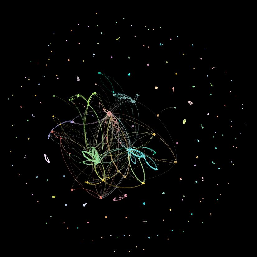
Last week I introduced our latest product: a network visualization of the Arctic Data Center repository where datasets in the repository are nodes, linked by contributors to those datasets. That network is much larger than its flip-flopped version, with people as nodes and datasets as links (3,792 nodes and 170,719 links versus 2,370 nodes and 7,530 links). Because the datasets-as-nodes networks is so much bigger, it’s hard to pick out the details of most of the components. So our first order of business this week is to delve a bit deeper into what the ingredients of the larger network look like.
Just as a reminder from last week, here’s what the whole network looks like:
Some network stats:
- Number of nodes: 3792
- Number of links: 170,719
- Average degree (the average number of links per node): 90
- Graph density (the percent of possible links that are actually present in the network): 0.024, or 2.4% realized links.
- Modularity (how clique-y the network is): 0.794 Very clique-y. Like, high-school clique-y.
- [Un]Connected components (the number of individual components): 167
- Average path length (the average number of nodes you have to pass through on your shortest path between any two nodes): ~4
That’s the network as a whole. Let’s dig a little bit deeper into that large structure in the center, the Giant Component:
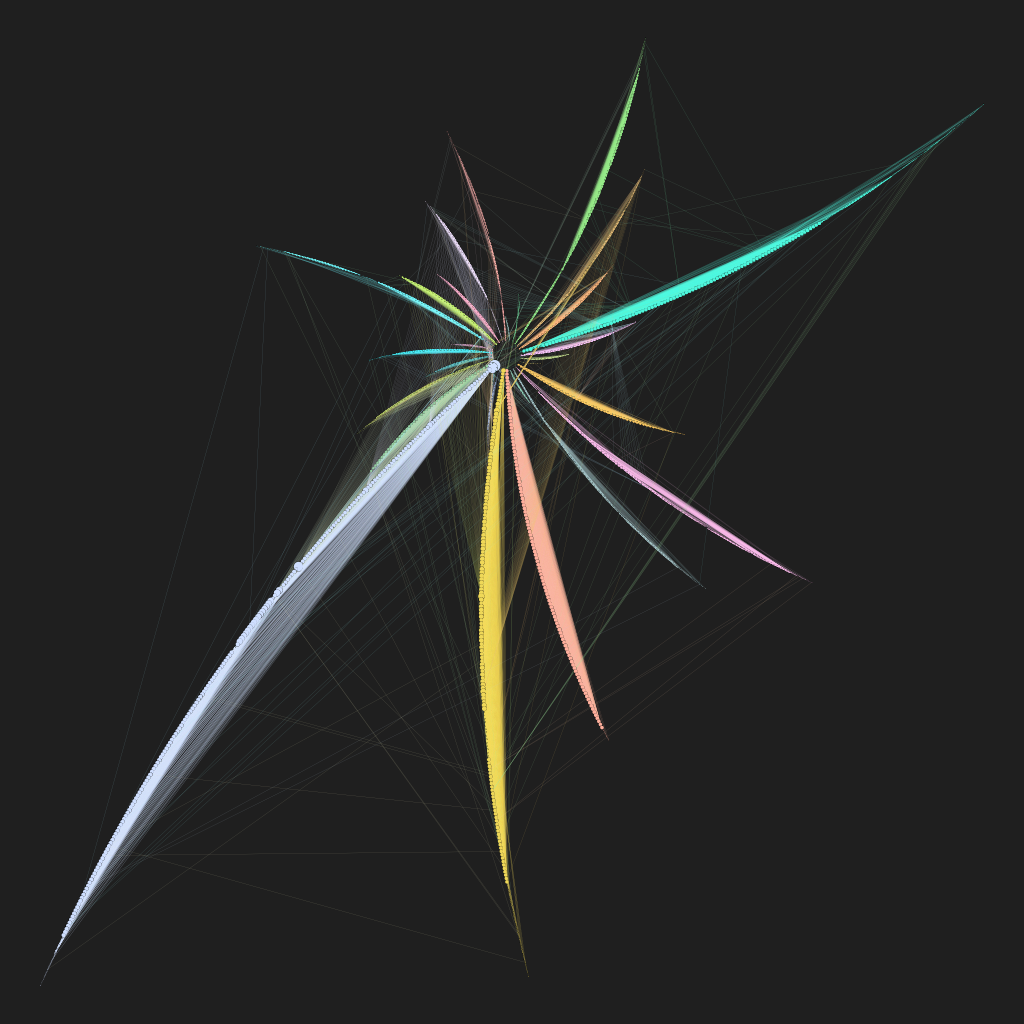
This visualization, rendered in Gephi, uses a layout algorithm called, appropriately, “radial axis.” It’s exactly the same information as displayed in the squiggly center of the first image, just arranged differently. Each of the “arms” is a community of datasets that are related to each other by contributors. If we’re thinking about disciplines as defined by datasets, like we were last week, we might think of the arms as data disciplines. Here’s a close-up on the center:
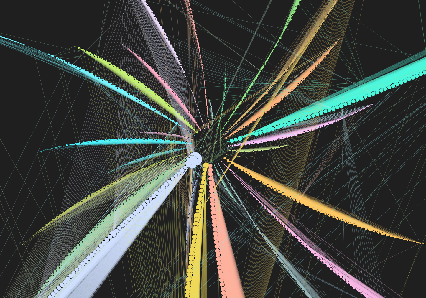
The nodes are sized by degree (the number of links connected to them), so those two big lavender nodes at 7 o’clock are very well connected. The teal arm at 2 o’clock has some highly-connected nodes near the center, but then several nodes with fewer connections. The entire orange arm at 4 o’clock isn’t very well connected to the rest of the giant component; we can see this because the nodes are relatively small.
Looking at the links, we see that most of the links connect nodes within a single community. The brush stroke of color filling in each arc of nodes is just a whole lot of links densely packed together. But we also see a spider-web of links that connect the different arms. These links represent people who work between data disciplines.
But the giant component isn’t the only interesting part of this network. Here’s a close-up on one of the smaller components:
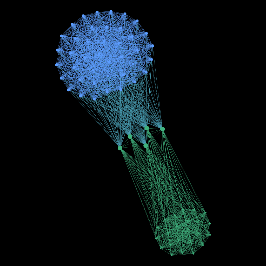
What’s going on here? We see two well-defined data disciplines–one in blue at the top and one in green at the bottom. These two communities represent groups of datasets connected by two distinct groups of contributors. Foreshadowing: if you’re interested in a particular dataset in the community at the top, there’s a good chance you might be interested in the other datasets in that same community. Similarly with a dataset in the group at the bottom. But this component is also connected by those five datasets in the middle, and contributors to those five central datasets work on datasets in both the top community and the bottom community. So, if you’re interested in Dataset A in the top community, not only will you probably be interested in the other datasets in the top community, but you also might be interested in one of the five central datasets, and even possibly in some of the datasets in the bottom community.
And we have arrived at The Great Reveal. The Really Cool Thing. The reason why network analysis is more than just an exercise in descriptive statistics, otherwise known as making pretty pictures. Network analysis is useful.
Imagine that you are a researcher with a particular question you want to answer. You search the Arctic Data Center archives, and find the dataset that will be perfect to answer your question. Unbeknownst to you, the archive holds a bunch of other datasets that also could be useful in answering your question. But maybe the keywords in the metadata are a bit off, or your search-term-foo isn’t quite at black-belt level. Before now, those useful other datasets might have remained invisible to you. But if DataONE’s software developers can figure out how to integrate modularity class into the search engine at DataONE, then when you search the DataONE archives we can provide suggestions for datasets that are connected to the one you found the old-fashioned way. Connected how? Connected by other people who thought, for whatever reason, that they were connected. And notwithstanding recent advances in machine learning, people are still way better than computers at sorting signal from noise.
Here’s how it works: All of the datasets in the top part of the network component visualized above belong to the same community. In programming terms, they have been assigned the same modularity class identifier. That’s what Gephi is using to determine which node gets what color–nodes in the same modularity class all get the same color. So when you search for a dataset and find one you like, say dataset “doi_10_18739_A26K65.xml”, DataONE’s search engine could look up the modularity class identifier, then give you a list of other datasets in the same modularity class. And just like that you have a list of the rest of the datasets in the same community.
Here is a list of the datasets in our network that have been assigned to the modularity class “72”.
- doi_10_18739_A2G65G.xml
- doi_10_18739_A26K65.xml
- doi_10_18739_A2GW6R.xml
- doi_10_18739_A2KW8F.xml
- doi_10_18739_A2NQ09.xml
- doi_10_18739_A2SH3M.xml
- doi_10_5065_D61R6NNG.xml
- doi_10_5065_D66T0JRJ.xml
- doi_10_5065_D6959FP6.xml
- doi_10_5065_D6GQ6VWS.xml
- doi_10_5065_D6J1019P.xml
- doi_10_5065_D6NZ85TB.xml
- doi_10_5065_D6PC30GB.xml
- doi_10_5065_D6XW4GXP.xml
- doi_10_5065_D6ZK5DSN.xml
With the network we’re building, if you find one, you’ve found them all.
(All of this is of course dependent on implementation. Are you listening Oh Great Software Developers in the Clouds? We’re not there yet, but we’re a lot closer than we were a month ago.)
And I think I will leave you here, to spend the week imagining the tantalizing possibilities. Stay tuned…
… Next week: The final products for this project are starting to take shape.